Conditional Formatting

Conditional formatting allows you to apply various formatting styles (color, font, decoration, gradient) to cells to work with data on the spreadsheet: highlight or sort through and display the data that meets the needed criteria. The criteria are defined by several rule types. The Spreadsheet Editor currently does not support creating and editing conditional formatting rules.

Rule types supported in the Spreadsheet Editor View mode are cell value (+formula), top/bottom and above/below average value, unique values and duplicates, icon sets, data bars, gradient (color scale), and formula-based rules.

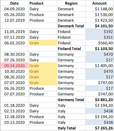
• Cell value to find needed numbers, dates, and text within the spreadsheet. For example, you need to see sales for the current month (pink highlight), products named “Grain” (yellow highlight), and product sales amounting to less than $500 (blue highlight).

  

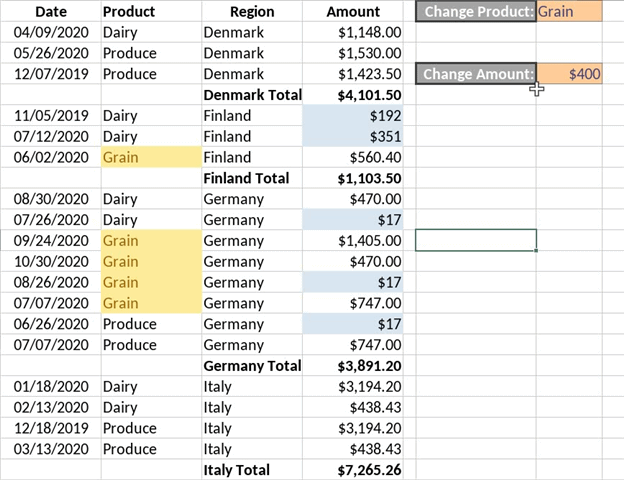
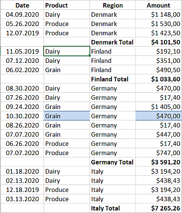
• Cell value with formula is used to display a dynamically changed number or text value within the spreadsheet. For example, you need to find products named “Grain”, “Produce”, or “Dairy” (yellow highlight), or product sales amounting to a value between $100 and $500 (blue highlight).

  

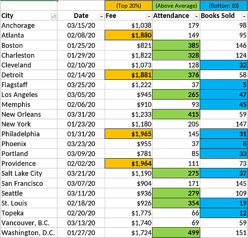
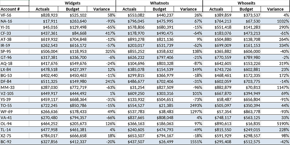
• Top and bottom value / Above and below average value is used to find and display the top and bottom values as well as above and below average values within the spreadsheet. For example, you need to see top values for fees in the cities you visited (orange highlight), the cities where the attendance was above average (green highlight), and bottom values for cities where you sold a small number of books (blue highlight).

  

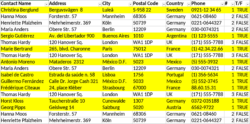
• Unique / Duplicates is used to display duplicate values within the spreadsheet and the cell range defined by the conditional formatting. For example, you need to find duplicate contacts. Enter the drop-down menu. The number of duplicates is shown to the right of the contact name. If you check the box, only the duplicates will be shown on the list.

• Icon set is used to show the data by displaying a corresponding icon in the cell that meets the criteria. The Spreadsheet Editor supports various icon sets. Below you will find examples for the most common icon set conditional formatting cases.

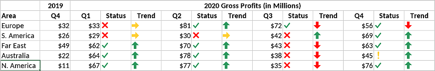
  • Instead of numbers and percent values, you see formatted cells with corresponding arrows showing you revenue achievement in the “Status” column and the dynamics for trends in the future in the “Trend” column.

    

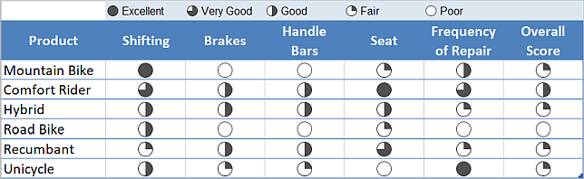
  • Instead of cells with rating numbers ranging from 1 to 5, the conditional formatting tool displays corresponding icons from the legend map at the top for each bike in the rating list.

    

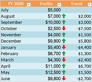
  • Instead of manually comparing monthly profit dynamics data, the formatted cells have a corresponding red or green arrow.

    

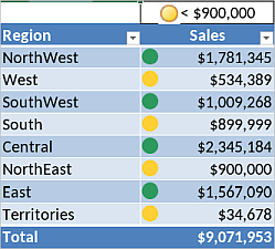
  • Use the traffic lights system (red, yellow, and green circles) to visualize sales dynamics.

    

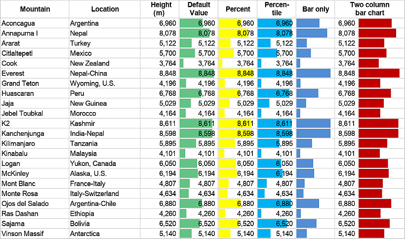
• Data bars are used to compare values in the form of a diagram bar. For example, compare mountain heights by displaying their default value in meters (green bar) and the same value in 0 to 100 percent range (yellow bar); percentile when extreme values slant the data (light blue bar); bars only instead of numbers (blue bar); two-column data analysis to see both numbers and bars (red bar).

  

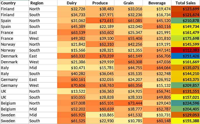
• Gradient, or color scale, is used to highlight values within the spreadsheet through a gradient scale. The columns from “Dairy” through “Beverage” display data via a two-color scale with variation from yellow to red; the “Total Sales” column displays data via a three-color scale from the smallest amount in red to the largest amount in blue.

  

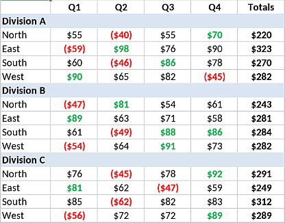
• Formula-based formatting uses various formulas to filter data as per specific needs. For example, you can shade alternate rows,

  

  compare with a reference value (here it is $55), and show if it is higher (green) or lower (red),

  

  highlight the rows that meet the needed criteria (see what goals you shall achieve this month, in this case, it is October),

  

  and highlight unique rows only